Disease ecology
Introduction
Disease ecology is a subset of the well established (and incredibly important) discipline of epidemiology. Epidemiology is the study of how diseases are distributed and transmitted through a population and/or the environment in an attempt to mitigate their spread and impact on humans, animals and plants. Disease ecologists and epidemiologists are not necessarily medical doctors but they do often work very closely with them in suggesting possible strategies when combatting disease outbreaks, for instance. Epidemiologists do this by studying how diseases are transmitted through a given population based on the disease’s characteristics. Epidemiologists often attempt to identify the cause of the disease in the population. Healthcare workers can then use this information to implement control measures to combat the disease’s progression through the population.
The disease ecologist’s job takes place at a slightly higher level - these researchers study the underlying principles of the disease which contribute to the disease’s spatial and temporal patterns. Theses researchers ask the why questions - they ask why a disease occurs in a particular region rather than the more mechanistic what or how questions that the epidemiologist might ask. Disease ecologists attempt to identify the population level principles and parameters of a given disease in a given scenario. This information could then be supplied to empidemiologists and medical practitioners for more lower level application.
We will discuss the theoretical intricacies and applications of disease ecology in the questions later in the practical but for now we will start by looking at a simple model of a disease entering a population.
The generic disease model
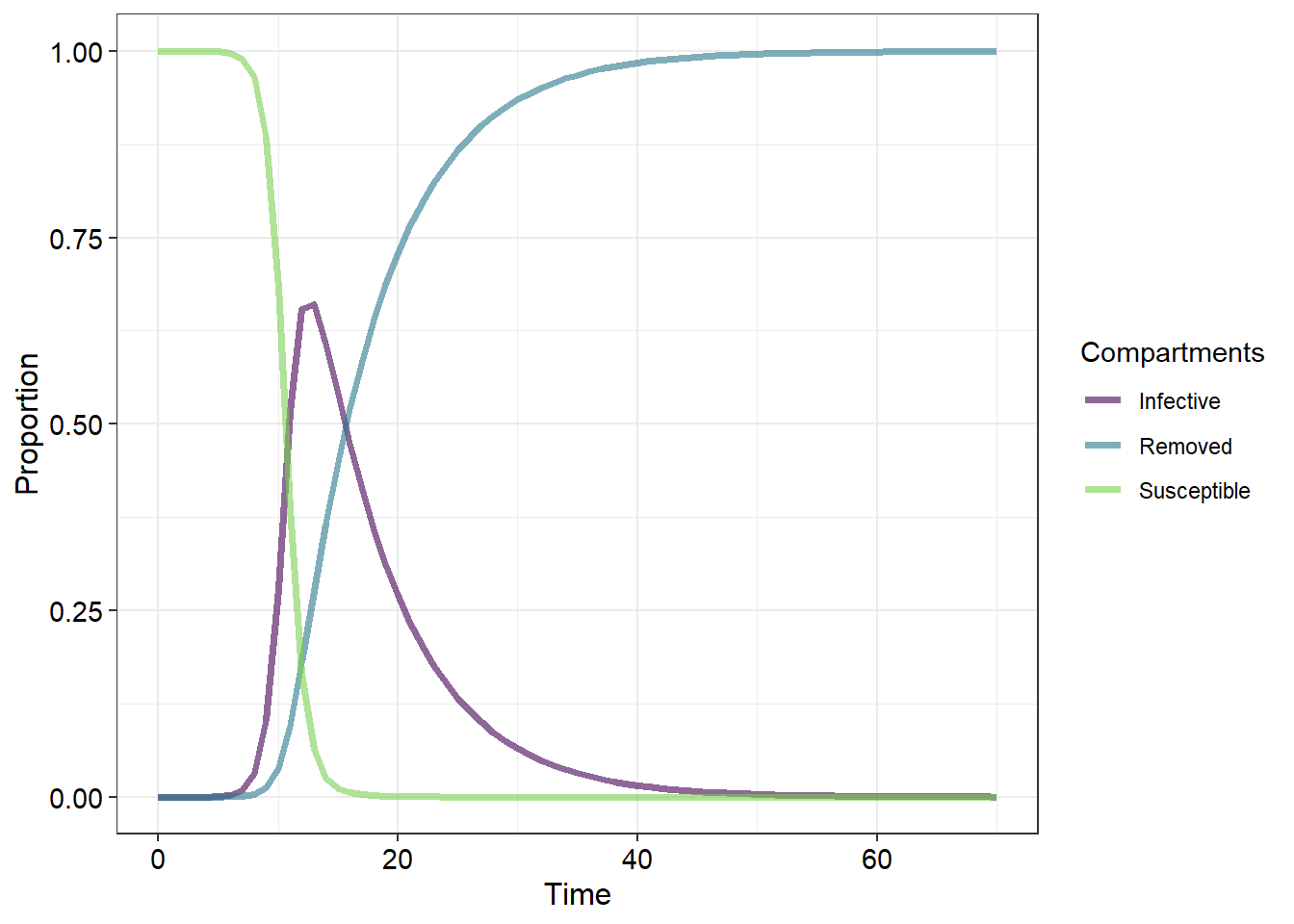
Populations exposed to some disease generally consist of at least three components - those which are uninfected by the disease but are nonetheless susceptible (termed susceptibles \(- S\)). These individuals cannot transmit the disease. Then there are those individuals which have become infected by the disease and can therefore transmit the disease (termed infectives \(- I\)). And then there are those individuals which are termed the removed individuals \((R)\). These are individuals which may or may not have the disease but for some reason do not become infectives. This could be due to several reasons - for example, they may possess inate, aquired or artificial immunity, or they may have died. There are others here but we will leave these examples out for later.
When using this \(SIR\) model we must be awear that there isn’t actually a “population growth equation”. This is because the overall population size does not change because we have included those individuals which have died in our population. Another important note is that there are three equations rather than just one. One equation models changes in susceptibles \(\frac{dS}{dt}\), the second models changes in infectives \(\frac{dI}{dt}\) and the third models the removed individuals \(\frac{dR}{dt}\).
The change in susceptibles is given by
\[ \frac{dS}{dt} = - \beta I S \]
Where \(\beta\) is a positive constant. This change in susceptibles then occurs at a the rate \(\gamma I\) where \(\gamma\) and so the rate of change of removed individuals is then given by:
\[ \frac{dR}{dt} = \gamma I \]
The change in infective individuals is then the differnence between these two rates of change:
\[ \frac{dI}{dt} = \beta I S - \gamma I \]
The values \(\beta\) and \(\gamma\) represent the number of contacts between suseptibles and the number of individuals that are removed per time period, respectively. For example, \(\beta = 2\) means that each time period each infective encounters two suseptibles while \(\gamma = 1.5\) means that every two days three individuals will transition from being infective to removed.
There are a few tricks that you should be awear of when carrying out your analyses. The first is that you should try to make the sum of the three components of your population equal to a whole decimal number (i.e. 1, 10, 100, 1000, etc.). The second is that you will have to start with some infectives in your population - these individuals will represent the disease carriers which act as the reserve pool from whence the susceptible individuals can be infected.
Let’s see how these parameters work together:
Download the basic SIR model app here.
Further exploring these parameters
Using \(\beta\) and \(\gamma\) we can calculate another important metric to describe our disease. The ratio \(\frac{\beta}{\gamma}\) (or alternatively \(\beta \times \frac{1}{\gamma}\)) represents \(c\), the contact number. The contact number represents aspects of both the population and the disease and is used to describe the contageousness of the disease and could alternatively be described as the number of close contacts per day per infective (\(\beta\)) times the number of days that an infective is infected for (\(\frac{1}{\gamma}\)) or more concisely the number of contacts that an infective has during the time that an individual is infective for.
What we have termed “removed individuals” is a broad category that contains several sub-categories. Broadly, these are members of the population which cannot become infective or susceptibles due to immunity or death. What we do not know from our current graphs is whether the population itself recovers or goes extinct. We also have not incorporated relapses (where infectives recover but remain susceptible).
Let us now examine a more complex disease model:

Here we have added a few new parameters that may better represent some of the more complex disease ecology scenarios. We have split up what was previously termed “removed” into dead and immune individuals and added several new pathways along which members of the population may progress with arrows indicating the direction in which the individuals can transition. The probabilities that an individual from one particular category will transition to another category are then represented by greek letters:
| Symbols | Descriptions |
|---|---|
| \(\beta\) | Number of contacts between susceptibles and infectives per day |
| \(\gamma\) | The inverse of the mean number of days an individual remains infective |
| \(\chi\) | Probability that a susceptible will develop immunity |
| \(\Delta\) | Probability that an infective will die |
| \(\epsilon\) | Probability that an immune will loose their immunity and become a susceptible |
| \(\sigma\) | Probability that an infective will become a susceptible |
But now that we have altered our initial SIR model (we now have an “SInImD” model) we will need to alter the inital equations which we used to calculate the changes in our population categories or compartments. Before we do that it is important to remember that because we are recording all of our deaths (and we are assuming that there are no births) we are not changing the population size. Thus our final equation must balance - the individuals which leave from one class must be added to another class. Thus, for our new “SInImD”" model we have:
\[
\frac{dS}{dt} = -\beta S I_n + \epsilon I_n - \chi I_m + \sigma I_n
\\
\frac{dI_n}{dt} = \beta S I_n - \gamma I_n - \Delta I_n - \sigma I_n \\
\frac{dI_m}{dt} = \gamma I_n + \chi S - \epsilon I_m
\\
\frac{dD}{dt} = \Delta I_n
\]
This is a lot of changes to our initial (and simpler) categorgy equations. We would likely spend a lot of time integrating these to calculate the changes in population category sizes at the different time periods.
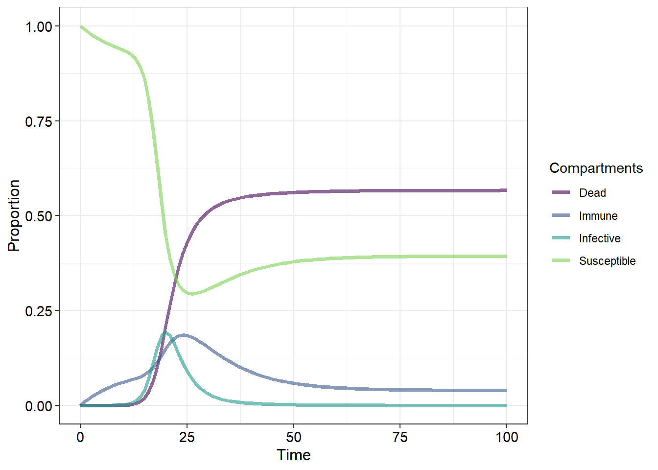
Now that we have developed a much more comprehensive model for our disease scenario you are ready to answer some questions using the interactive app.
Download the more complex SIR model app here
Worksheet questions
Basic modelling of susceptibles, infectives, and removeds
Use the first app to answer the following questions
Question 1
- Describe how \(\beta\) influences the shape of the three curves (3)
- Describe why the observed responses are the case (4)
Question 2
Give the biological relevance of \(\gamma\) (3)
Question 3
- Describe how changning \(\gamma\) influences the shape of the three curves (3)
- Describe why the observed responses are the case (4)
Question 4
How do both \(\beta\) and \(\gamma\) influence the B : K ratio (6)
Complex modelling of susceptibles, infectives, and removeds
Use the second app to answer the following question
Question 1
Copy the following table onto your exam pad and fill in the three empty columns by adjusting the parameters in the complex SIR app (6 x 3 = 18)
| Parameter | Compartment | Direct or indirect effect by parameter on compartment | Direction of the affect on the compartments (either positive or negative) | Parameter effect on the shape of the compartment response curve |
|---|---|---|---|---|
| \(\beta\) | Dead | |||
| Immune | ||||
| Infective | ||||
| Susceptible | ||||
| \(\gamma\) | Dead | |||
| Immune | ||||
| Infective | ||||
| Susceptible | ||||
| \(\chi\) | Dead | |||
| Immune | ||||
| Infective | ||||
| Susceptible | ||||
| \(\delta\) | Dead | |||
| Immune | ||||
| Infective | ||||
| Susceptible | ||||
| \(\epsilon\) | Dead | |||
| Immune | ||||
| Infective | ||||
| Susceptible | ||||
| \(\sigma\) | Dead | |||
| Immune | ||||
| Infective | ||||
| Susceptible |
Coding questions
Below is the code required to produce Figure 1. Modify this code by incorporating the necessary equations and any aesthetic/thematic changes in order to produce a figure which matches the “SInImD” model pictured below (10)
library(desolve)
library(dplyr)
library(tidyr)
library(ggplot)

library(viridis)

sir <- function(time, state, parameters) {
  with(as.list(c(state, parameters)), {
    dS <- -beta * S * I
    dI <-  beta * S * I - gamma * I
    dR <-  gamma * I

    return(list(c(dS, dI, dR)))
  })
}


init <- c(S = 1-1e-6,
          I = 1e-6, 0.0)
parameters <- c(beta = 1.4247,
                gamma = 0.14286)
times <- seq(0, 70, by = 1)
out <- ode(y = init,
           times = times,
           func = Sir,
           parms = parameters)

out_df <- as.data.frame(out)
colnames(out_df) <- c("time", "Susceptible", "Infective", "Removed")

out_df <- out_df %>% gather(key = "Compartments", value = "Proportion", -Time)

ggplot(data = out_df) +
  geom_line(aes(x = Time,
                y = proportion,
                colour = Compartments),
            size = 1.25,
            alpha = 0.6) +
  scale_color_viridis(discrete = FALSE, end = 0.8) +
  theme(axis.title = element_text(colour = "black",
                                  size = 12),
        axis.text = element_text(colour = "black",
                                 size = 11),
        legend.title = element_text(colour = "black",
                                  size = 12),
        legend.text = element_text(colour = "pink",
                                 size = 11))
- Some diseases remain dangerous long after the infected individual has died. Depending on the number of dead individuals the disease “reservoir” in the area increases. Living susceptible individuals may come into contact with this reservoir and become infectives themselves. Using the diagram below which indicates how susceptibles may become infectives based on the number of dead individuals develop a new equation and parameter and produce a figure that incorporates the reservoir into the disease model (15)
Application questions
One of the most ecologically important diseases in KwaZulu-Natal is the rabies virus. After doing some reading on the disease choose one of the two disease models used in this practical which best represents how this disease progresses. Give a brief explanation on why you chose your particular model (4)
In order to prevent a disease from infecting and becoming established in a population the population needs to be immune to the disease. There are many sources of immunity which are broadly classified into passively, naturally or artificially aquired. For each of these three categories of immunity identify and briefly describe three examples (9)
When managing disease control any population an important consideration is something termed the population’s critical size. Define this term in the context of population and community ecology and discuss using references to real world applications from the scientific literature how conservation managers can protect populations from disease outbreaks (10)
Discuss the differences between the disciplines of epidemoilogy and disease ecology with reference to scientific articles. Discuss how both disciplines can work together to allow humans to better manage and mitigate disease in both animal and human populations (10)