Population Growth

Introduction

When a species is of conservation concern, we are interested in whether populations of the species can persist in the long term. In order to examine population viability (a measurement of whether a species will persist through time), we can use demographic information to model population dynamics.

Usually we start with the idea that in any population, the number of individuals at any particular time is governed by the initial population size, $N_0$, and the number of births, deaths, immigrations, and emigarations that occur. We can describe this kind of population using the following diagram:

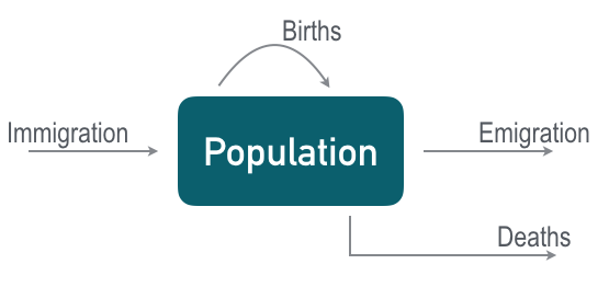
Given this scenario we could use the equation

$$N_{t+1}=N_t+B-D+I-E$$ to describe how the population changes between time periods. Here $N_t$ represents the number of individuals in the population, $B$ represents the number of births, $D$ the number of deaths, $I$ the number of immigrations, and $E$ the number of emmigrations. In the simplest approach, we can use a disctrete-time model and demographic information to predict the expected size of a population over time.

The above equation has several sources of external variability due to external influences and so for simplicity we will consider a closed population, where there are no immigarants joining the population or emmigrants leaving the population. In our example only births and deaths will affect the number of inidividuals in the population.

To further simplify our model, we will not explicitly address deaths. Instead we examine suvivorship, $S$, or the per capita probability of suriving in a particular timestep. $S$ is still calculated with the per capita death rate ($d$) in mind:

$$S=1-d$$ This equation means that the probability that an individual will survive ($S$) plus the probability that an individual will die ($d$) must add to one. From this we can estimate the number of individuals alive at time $t+1$ as $N_t\times S$. Then population size in each timestep is a function of the population size at the time before ($N_t$), survivorship ($S$), and the per capita birth rate ($b$) as shown in the equation below.

$$N_t+1=N_t[S+b]$$

Use the Exponential growth: Births and survivorship app to study this equation a little further. Use this app to answer the questions on the prac sheet.

Download the exponential growth: Births and deaths app here

Futhermore, in order for a population to remain viable in the long term, survivorship and births must be balanced so that $S+b\ge 1$. The term $\lambda$ is often used to summarize the sum of per capita survivorship and births:

$$\lambda =S+b$$

So, instead of changing $S$ and $b$ independently, we can use $\lambda$ in our model to summarize the dynamics of the population. Use the Exponential growth: Lambda app to answer the next set of questions on your prac sheet.

Download the exponential growth: Lambda app here

A bief note about calculus in population ecology and R

An important aspect of any population study is the rate of change of a population’s size between two time periods $\left(\frac{dN}{dt}\right)$. Going back to MATH150 you’ll hopefully remember that the term for this is differentiation. Some equations are pretty easy to differentiate (a cubic function (the logisic growth equation is a variation of this) differentiates to a parabolic function) but many of the equations used in population ecology are a little more complicated than this and so differentiating more complicated equations becomes much more tricky and likely goes beyond the scope of MATh150. Fortunately for us, R has several packages which takes care of this differentiation stuff for us! One such package is deSolve. In later practicals we will learn how to use this package but for now we will just focus understanding the relationship between the variables involved in the equations rather than computing the relationship ourselves.

Worksheet questions

Coding questions

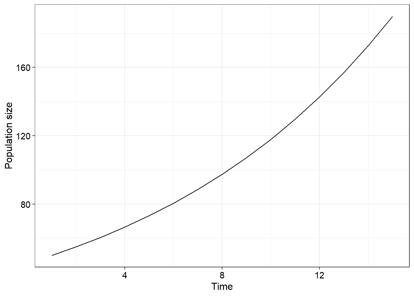
1. The following code is mostly complete except for a few errors which result in a completely incorrect output. Identify the errors (there are four in total worth one mark each) to produce a plot that matches the one below it. You can copy this code directly into RStudio. Edit the code until it produces the desired output and then copy the corrected code into a word document. In your word document also list each of the errors and briefly (no more than one sentence) describe how you fixed the error (10)

  
  N0 <- 50    # The intitial population size
  years <- 30    # The number of time steps
  lambda <- 1.4     # The population growth rate, lambda
  N <- c(N0, rep(0, times = years - 1))  # Create an open vector for data
  
  #Run a loop that considers each time step (t) as a function of the time step before it (t-1) and lambda
  for (t in 2:years) {
    N[t] <- N[t - 1]*(lambda)
  }
  
  time <- seq(from=1, to = years, by = 1)  #Create a vector of time steps for plotting
  plot_df <- data.frame(Size = N, Time = time)
  
  ggplot(data = plot_df) + 
    geom_line(aes(x = Time, y = Size)) + 
    labs(x = "Time") 
         theme_bw() + 
         theme(axis.title = element_text(colour = "black", 
                                         size = 12), 
               axis.text = element_text(colour = "black", 
                                        size = 11), 
               legend.title = element_text(colour = "black", 
                                           size = 12),
               legend.text = element_text(colour = "black", 
                                          size = 11))

2. Similar to the above scenario, the following code also contains several errors. However, there are two “fatal” errors in this scenario - that is the code does not successfully compile. Present your corrections in the same manner as described in the previous question (10)

  N0 <- 25    # The intitial population size
  years <- 15    # The number of time steps
  r <- 1.01     # The population growth rate, lambda
  K <- 90

  N <- rep(0, times = years+1)  # Create an open vector for data

  years <- seq(from = 0, 
               to = years, 
               by = 2)

    for (i in 1:length(N)+1) {
      
      N[i] <- K/(1+((K-N0)/N0)*exp(-r*years[i]))
      
    }
    
    ggplot() + 
      geom_point(aes(x = years, y = N)) + 
      geom_line(aes(x = years, y = N)) + 
      labs(x = "Years") + 
      theme_bw() + 
      theme(axis.title = element_text(colour = "black", 
                                      size = 12), 
            axis.text = element_text(colour = "black", 
                                     size = 11), 
            legend.title = element_text(colour = "black", 
                                        size = 12),
            legend.text = element_text(colour = "black", 
                                       size = 11))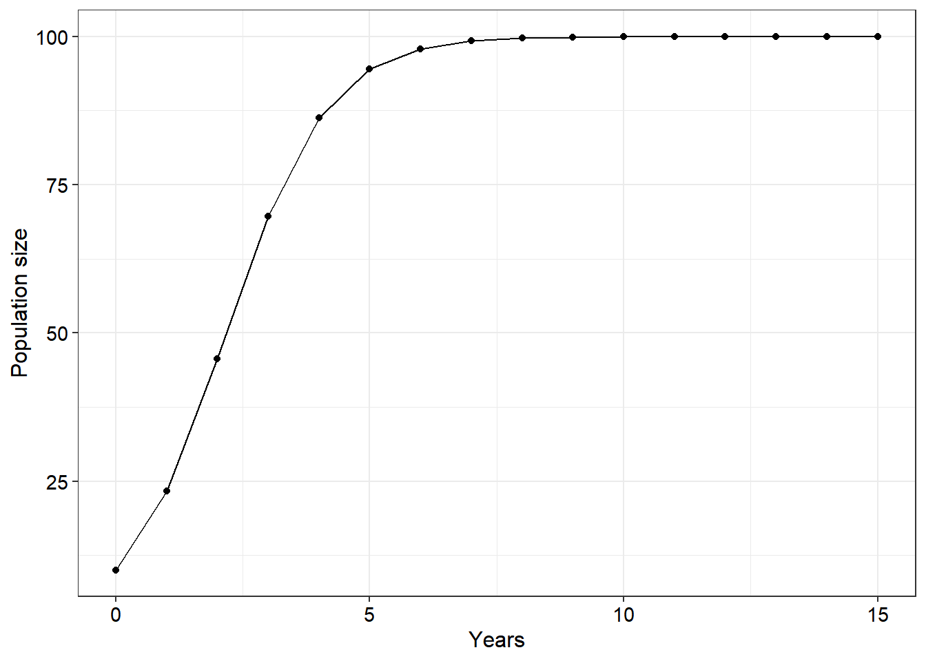

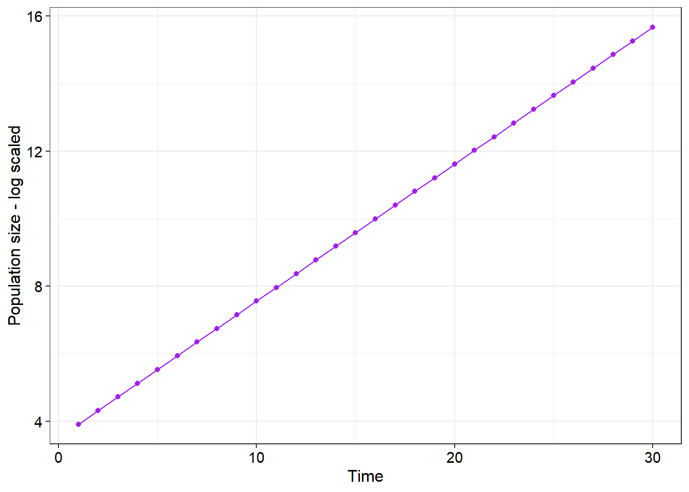
3. Bonus challenge. The following plot is similar to the first plot, however, there are some important changes that need to be made to the figure output section in order to obtain the desired output. Look carefully at the output for some hints and suggestions. You will also need to include a new geom layer (5)

  
   N0 <- 50    # The intitial population size
  years <- 30    # The number of time steps
  lambda <- 1.4     # The population growth rate, lambda
  N <- c(N0, rep(0, times = years - 1))  # Create an open vector for data
  
  #Run a loop that considers each time step (t) as a function of the time step before it (t-1) and lambda
  for (t in 2:years) {
    N[t] <- N[t - 1]*(lambda)
  }
  
  time <- seq(from = 1, 
              to = years, 
              by = 1)  #Create a vector of time steps for plotting
  plot_df <- data.frame(Size = N, Time = time)

  ggplot(plot_df) + 
    geom_line(aes(x = Time, y = Size)) + 
    labs(x = "Time") 
         theme_bw() +
         theme(axis.title = element_text(colour = "black", 
                                         size = 12), 
               axis.text = element_text(colour = "black", 
                                        size = 11), 
               legend.title = element_text(colour = "black", 
                                           size = 12),
               legend.text = element_text(colour = "black", 
                                          size = 11))

Application questions

1. Find three peer reviewed examples where studies have investigated populations growing exponentially and logistically. Give the citation of the paper and the study species. For the three logistically growing populations indicate what environmental factors that the reasearchers linked the carrying capacity to (9)
   
2. Give three factors that could influce both the birth and the survivorship rates (and ultimately $\lambda$) for a given population. Give reasons for your answers (6)
   
3. About 160 years ago an alien plant species was introduced to KwaZulu-Natal after a ship carrying a delivery of exotic plants from Mexico to China docked at Port Natal harbour. Trade reports stated that 3 specimens of Lantana camara were sold to a local wealthy family to “beautify” their garden. A recent survey of densities of L. camara in South Africa reported that aprroximately 2 000 000 ha have been invaded by the plant. Assuming that at the time L. camara was introduced into KwaZulu-Natal 1 ha was invaded by the plant, calculate the intrinsic population growth rate between the species’ introduction and the date that the article was published. Show all your working (6)
   
4. Based on the brief discussions in this article what kind of growth pattern (exponential or logistic) do you think L. camara likely demonstrates? (4)
   
5. There are two methods one can use to model population growth. They are discrete and continuous growth. In your own words discuss the theoretical and applied differences of these two methods. You may include examples and references to scientific publications and equations to support your answer (5)