BIOL 305 - Population and community ecology > Practicals > Practical 5 > Common resource competition

Common resource competition

Introduction

In the logistic model of population growth we saw that resource limitation can be included in an abstract way by including a carrying capacity for a population. But, what if there are also other species competing for the same resources? Depending on the strength of competition, competing species can reduce equilibrium population abundance below the carrying capacity. To jog your memory, here is the discrete-time version of logistic growth:

$N_{t + 1} = N_{t} + r N_{t} (1 - \frac{N_{t}}{K})$

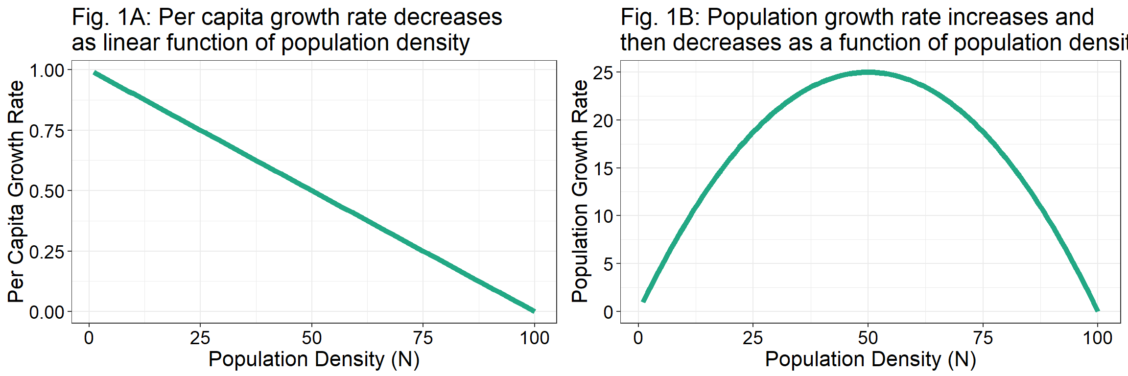
where $r$ is the intrinsic per capita growth rate, $N$ is the population abundance, and $K$ is the carrying capacity. The effect of $(\frac{N}{K})$ is intraspecific competition (density-dependence) – the closer $N$ comes to $K$ , the slower the population grows. However, carrying capacity is a notoriously difficult term to define and quantify. Peter Chesson (2000) describes a more intuitive way to think about population growth by assuming that “per capita growth rates are linear decreasing functions of the density” of the population (Figure 1A). When this is the case, population growth rate starts low when a species is at low abundance (low $N$ , high $r$ ), increases to a maximum when a species reaches a moderate abundance (medium $N$ , medium $r$ ), and then decreases as the population reaches a high density (high $N$ , low $r$ ) (Figure 1B).

So, we can rewrite the logistic growth equation as:

$N_{t + 1} = N_{t} + r N_{t} (1 - α N)$ where $α$ is the absolute effect of intraspecific competition, and is equal to $1 / K$ . If $α$ is really small, then intraspecific competition (density-dependence) is negligible. If $α$ is very large, then intraspecific competition strongly limits population growth and size. The reason we go to all this trouble to rewrite the logistic growth equation is to make it easier to include the effects of other species on population growth. But first, let’s make the equation a little more simple by writing it in terms of population growth rates $(\frac{d N}{d t})$ , rather than population size, and by adding subscripts to denote we are talking about species $i$ :

$\frac{d N_{i}}{d t} = r N_{i} (1 - α_{i i} N_{i})$

Notice how we have now dropped the $t$ subscripts because we are now defining population growth at any instantaneous point in time. Also notice that we added two $i$ subscripts to $α$ . Here $α_{i i}$ reads as the effect of species $i$ on species $i$ .

To include the effect of another species, we assume that growth is further limited by a simple function of the number of the other species, $α_{i j} N_{j}$ , where $α_{i j}$ reads as: “the effect of species $j$ on species $i$ ”. Putting it all together, we can write equations for a two-species community as:

$\begin{aligned} \frac{d N_{1}}{d t} & = r_{1} N_{1} (1 - α_{11} N_{1} - α_{12} N_{2}) \\ \frac{d N_{2}}{d t} & = r_{2} N_{2} (1 - α_{22} N_{2} - α_{21} N_{1}) \end{aligned}$

where the new parameter $α_{21}$ is the absolute interspecific competition coefficient describing the effect of species 2 ( $N_{2}$ ) on species 1 ( $N_{1}$ ). Recall that the fundamental requirement for species coexistence is that each species must be able to increase from low density (i.e., when it is rare in the community), implying that intraspecific competition must be greater than interspecific competition. Put more simply, each species must limit individuals of its own species more than it limits individuals of other species.

Because the $α$ ’s control intra and interspecific competition in the Lotka-Volterra model, we can state the criterion for coexistence mathematically as:

$α_{j j} > α_{i j}$

which simply states that species $j$ cannot competitively exclude species $i$ if the effect it has on itself is greater than the effect it has on species $i$ . For a two species community, the coexistence is stable if, and only if:

$α_{11} > α_{21} AND α_{22} > α_{12} .$

The multispecies equation

Just in case you ever see this in a paper, it is often written in the multispecies case as:

$\frac{d N_{i}}{d t} = r_{i} N_{i} (1 - α_{i i} N_{i} - \sum_{i \neq j}^{S} α_{i j} N_{j})$

where $S$ is the number of species in the community.

Table of parameters and states

To keep everything clear, here is a table of model states and parameters.

Parameter	Definition
$N_{i}$	The abundance (or biomass, depending on units) of species $i$
$r_{i}$	Species $i$ ’s intrinsic per capita growth rate
$α_{i i}$	Intraspecific competition coefficient (effect of species $i$ on itself)
$α_{i j}$	Interspecific competition coefficient (effect of species $j$ on species $i$ )

Parameter exploration

Download the common resource competition app here and answer the first section of the Worksheet questions.

Incorporating carrying capacity

By now you should understand that carrying capacity plays a pretty important role. In the previous examples we incorporated carrying capacity into the model by accounting for the effect of species 1 on species 1 and species 2 on species 2. But there are other methods which can be more appropriate depending on data availability. Suppose we have two species ( $N_{1}$ and $N_{2}$ ) utilising one set of finite resources ( $K$ ). It is likely that the set of finite resources cannot sustain both species 1 and species 2 at the same number - one species would likely require more resources than the other species and so we would have two carrying capacities ( $K_{1}$ and $K_{2}$ ) and two different population growth rates ( $r_{1}$ and $r_{2}$ ). From this we can develop two equations to model the two species’ population sizes through time:

$N_{1, t + 1} = N_{1, t} + r_{1} N_{1, t} \frac{K_{1} - N_{1, t}}{K_{1}}$ $N_{2, t + 1} = N_{2, t} + r_{1} N_{2, t} \frac{K_{2} - N_{2, t}}{K_{2}}$

This is a step in the right direction but what is missing is the competitive ability of the two species. By incorporating carrying capacity into our equations we have successfully accounted for the effect that conspecifics (individuals of the same species) have on each other but we have not accounted for the interspecific competitive effects (i.e. increases in species 2’s population on the growth rate of speices 1). As the growth rate is dependent on the resources available to the population in question a good place to incorporate this competitive effect would be at around $K_{1} - N_{1, t}$ term. We could simply minus $N_{2, t}$ as well but it is also likely that the two species do not have exactly the same effect on the available resources. Thus we can incorporate a competition coefficient modifier to this term and so the numerator would then be $K_{1} - N_{1, t} - a_{12} N_{2, t}$ .

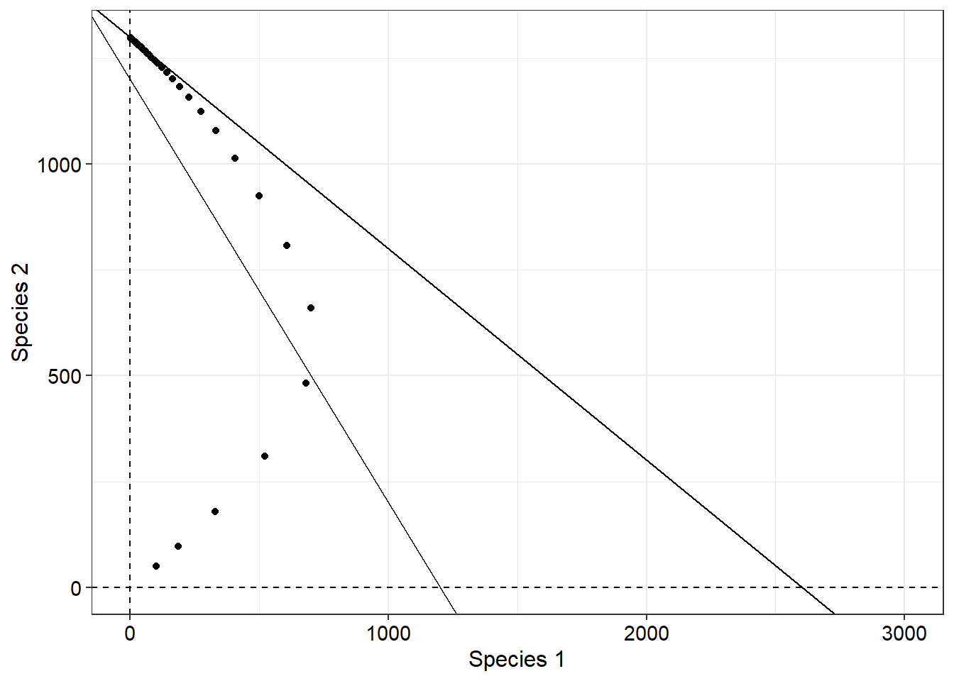
Often ecologists are interested in whether one species will outcompete the other or whether the two species will be able to coexist. To investigate this we can consider scenarios when there will be no change in the population size from time $t$ to time $t + 1$ . That is $N_{1, t + 1}$ equals $N_{1, t}$ . This can be true for a number of scenarios such as when $r = 0$ or $N_{1, t} = 0$ . Those are rather simple scenarios but there will also be no change in the population when $K_{1} - N_{1, t} - a_{12} N_{2, t} = 0$ . We can easily convert this equation to a linear equations of the form $y = a + b x$ - the equation for a straight line. This line can then represent the situations where species 1 will not grow and so we call it the zero net growth isocline (ZNGI). We can do a similar thing for species 2. The points where these lines intersect the $x$ and $y$ axes can provide us with important information. When $N_{1, t} = 0$ we have the situation where $K_{1} = a_{12} N_{2, t}$ which translates to $N_{2, t} = \frac{K_{1}}{a_{12}}$ . Similarly if $N_{2, t} = 0$ then $N_{1, t} = K_{1}$ . These equations state that if there are $\frac{K_{1}}{a_{12}}$ individuals of species 2 then there will be no resources for species 1 and so species 1 will be excluded. Similarly, if there are no individuals of speceis 2 then species 1 will reach its carrying capacity. This might seem quite complicated butyou should be familiar with these methods from MATH 150.

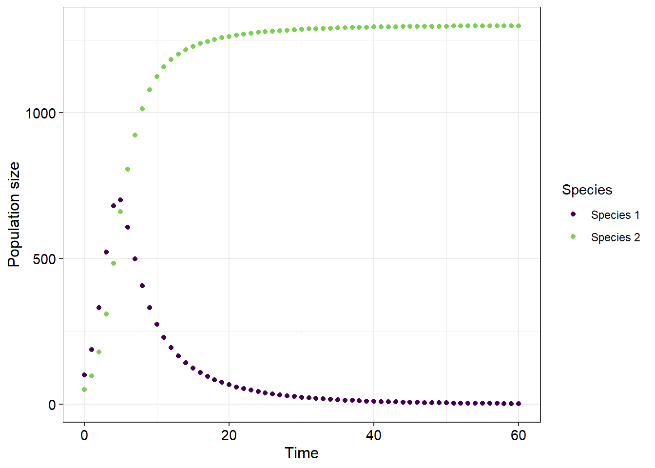
Below are the two species’ population sizes through time together with a plot of the populations’ ZNGIs.

Parameter exploration

Download the common resource competition ZNGI app here and answer the second section of the Worksheet questions.

Worksheet questions

Common resource competition

Question 1

Use only Figure 1 of the app to answer the following questions

Under what conditions will one species exclude the other (4)

Question 2

Under what conditions will both species coexist (4)

Question 3

Are there a set of parameters where both species in this model will become extinct? Explain your answer (6)

Use both Figure 1 and Figure 2 to answer the following questions

Set your parameters to $α_{i i}$ = 0.6, $α_{j i}$ = 0.3, $α_{i j}$ = 0.5, $α_{j j}$ = 0.1

What does it mean that ajj = 0.1 (2)
What does it mean that aji = 0.3 (3)
Describe the output of Figure 2 (2)

Question 4

Describe what the second plot represents and give reasons for why this kind of plot is useful (4)

Carrying capacity and interspecific competition

Question 1

Consider Figure 1 from both this and the previous app to answer the following question

Discuss how this plot differs from the first plot in the previous app (6)

Question 2

Consider Figure 1 and 2 from this app to answer the following question

Under what conditions would you find a) stable and b) unstable competitive exclusion (6)
Under what conditions would you find these two populations coexisting in a stable equilibrium (4)

Coding questions

For now we will only work with the carrying capacity example rather than the inter/intraspecific example.

The following code contains all the code necessary for producing the desired plot output. All the parameters are set correctly and the ggplot2 code is correctly written. What is missing is the for loop code to calculate the population sizes for the two populations and the construction of the dataframe to contian the data for the final plot. Modify the following code by correctly incorporating the for loop and building the required dataframe (15)


N01 <- 100
N02 <- 50
K1 <- 1200 
K2 <- 1300
r1 <- 1
r2 <- 1 
a12 <- 1 
a21 <- 0.5 
time <- seq(from = 0, to = 60, by = 1)

N1 <- c(N01, rep(0, length(time)-1))
N2 <- c(N02, rep(0, length(time)-1))

ggplot(df2) + 
  geom_point(aes(x = Time, y = Number, colour = Species)) + 
  theme_bw() + 
  theme(axis.title = element_text(colour = "black", 
                                      size = 12), 
            axis.text = element_text(colour = "black", 
                                     size = 11)) + 
  scale_color_viridis(discrete = TRUE, end = 0.8) + 
  labs(y = "Population size")

Your second coding task for this practical will be to generate the desired ZNGI curves. You will have to think carefully about how to produce the desired output as only the equation parameters will be provided (25)


N01 <- 100
N02 <- 50
K1 <- 1200 
K2 <- 1300
r1 <- 1
r2 <- 1 
a12 <- 1 
a21 <- 0.5 
time <- seq(from = 0, to = 60, by = 1)

N1 <- c(N01, rep(0, length(time)-1))
N2 <- c(N02, rep(0, length(time)-1))

Application questions

The models used in this practical have several key assumptions. Identify and discuss these assumptions with reference to the model parameters and provide suggestions on how these assumptions can be improved upon (6)
When species compete with other species there are several outcomes that can occur. Give 2 biological examples with reference to scientific publications of facilitation, exclusion, and co-occurrance (12)
The central aspect of either of the two competition equations used in this practical are the competition coefficients. Discuss how these values could be estimated using field methods (6)
Conservationists and ecologists often need to employ these (or very similar) equations when managing conservation areas. Another application of these methods is when predicting the effects of new species introductions on species currently inhabiting a given area. In the form of a one page essay citing at least eight difference scientific publications, discuss the real world applications of these competition type population models to invasive species introductions and control/management and conservation reserves where several species depend on a common resource which could result in competitive exclusion or facilitation (16)