BIOL 305 - Population and community ecology > Practicals > Practical 6 > Predator - prey interactions

Predator - prey interactions

Introduction

In the Lotka Voterra Competition exercise, we saw that the dynamics of any given species can be influenced by those of other species which are competing with it for resources. This often takes place within a particular trophic level. In nature, population dynamics are also regulated by species across trophic levels. For example, the dynamics of predator populations are influenced by how many prey individuals are in the community. The Lotka-Voterra Predator-prey equations are a pair of differential equations that describe the population dynamics of one species at one trophic as a function of the dynamics of species on the other trophic level. Although it is most communly discussed in a “predator-prey” context, the framework here can also be applied to plant-herbivore, parasites-host, or any other trophic interaction.

Exponentially growing prey

The simplest Lotka-Volterra predator-prey equation considers a prey or victim species $V$ that grows exponentially at a rate $r$ , and shrinks as it gets consumed by predators $V$ , which attack the prey they encounter at a per-capita (i.e. dependent on the number of predators and prey) rate $α$ :

$\frac{d V}{d t} = r V - α V P$

The population of the predator $V$ grows as it converts the prey it consumes into new predator individuals at the rate $b$ , and shrinks due to a constant per-capita mortality rate $d$ :

$\frac{d P}{d t} = β α V P - d P$

Let’s take a look at what this model implies. When there are no predators in the community (i.e. $P = 0$ ), the prey species $V$ grows due to simple exponential growth. If there were limiting resources then the prey would grow until its carrying capacity but we will ignore that aspect in this example for simplicity. Conversely, when there are no prey individuals in the community (i.e. $V = 0$ ), the predator popultion has no way to grow and exponentially declines at a rate $d$ .

The rate of growth of the predator population increases when prey are abundant and predators are few. On the other hand, when there are plenty of predators, the prey population suffers and cannot grow very quickly. We can get some suggestion that this predator-prey relationship might lead to some sort of population cycling - as the prey population grows, so too does the predator popuplation, which in turn reduced the number of prey which will in turn reduce the number of predators allowing the prey to increase once more.

As expected, cyclic population dynamics are common in predator-prey systems:

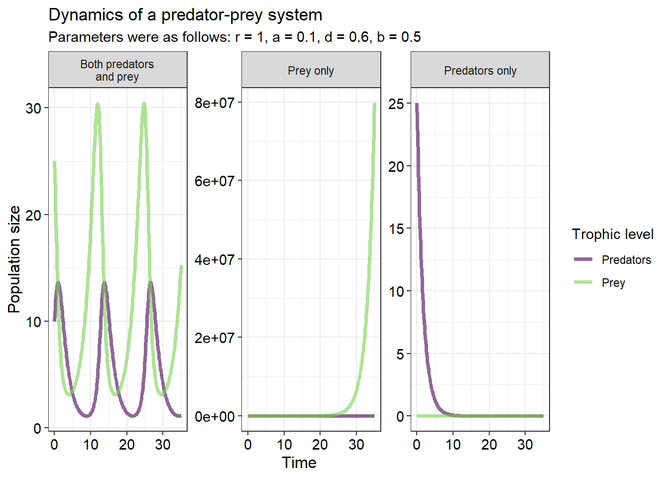
In the first plot above, the system begins with 25 prey and 10 predators - cyclic dynamics shortly ensue. In the middle panel, there are no predators in the beginning, so the prey population simply grows exponentially. In the third panel, there are no prey individuals in the system- so, the predator population shrinks exponentially to zero.

Logistically growing prey

In the previous model, prey experience exponential growth when predators are absent - in other words, the predators are the only factor regulating the prey population’s dynamics. Of course, this doesn’t generally happen in nature - even when predators are absent, a prey population will eventually level off at some carrying capacity dictated by their habitat’s resources.

To incorporate this aspect into our equations we can modify the above prey equation by incorporating density-dependent growth simply by adding a carrying capacity in the same was as we did in the Logistic Growth exercise:

$\frac{d V}{d t} = r V - α V P - c V^{2}$

Where the value of the carrying capacity can be calculated as $K = \frac{r}{c}$ . So if you wand a very large $K$ then make $c$ very small. We keep the predator population dynamics the same as before:
$\frac{d P}{d t} = b a N P - d P$

With these new equations, when predators are absent from the community, the prey species grows exponentially but then is restricted by its own abundance in a similar manner to how the logistic growth equation would function. One possible outcome in this case is stabilised population cycles - in other words, the predator and prey populations can cycle up and down until they reach a joint equilibrium:

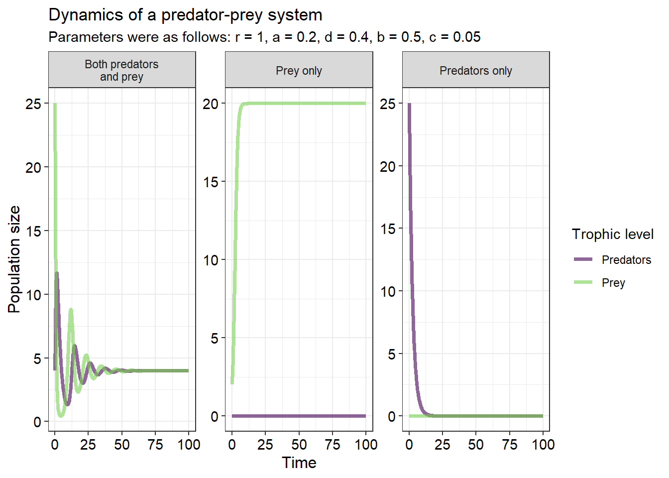
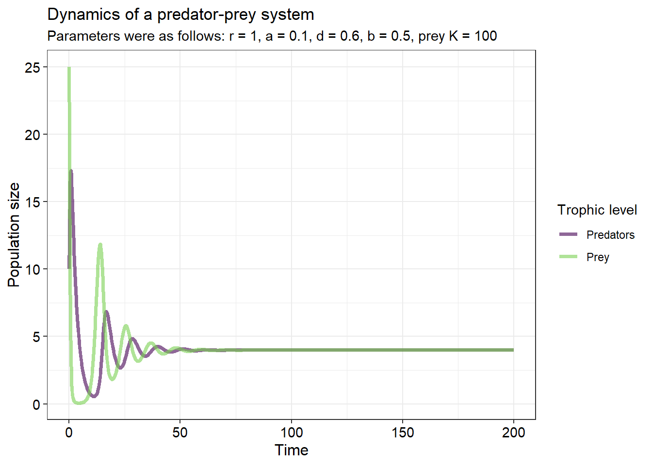
Note that in the middle graph, the prey population grows logistically to its carrying capacity of 100 when no predators are present. If we run this system out longer, we see that the populations eventually stop cycling as they reach an equilibrium when both predator and prey are present in the system:

Parameter exploration

Download Lotka-Voltera predator prey app here and answer the questions on the prac worksheet.

Worksheet questions

Question 1

An important starting point for any model is understanding what the different aspects of the equation represent. One can access this information from the units that a particular parameter is measured or reported in. Give the units of:

$α$ (3)
$β$ (3)

Question 2

Briefly explain how the term $c V^{2}$ produces similar outcomes to the term $(1 - \frac{N}{K})$ (2)
Why do we only incorporate carrying capacity (in the form $(\frac{r}{c})$ ) into the prey population growth equation but not into the predator population growth equation (3)

Question 4

Describe how the parameters of the predator equation interact with the prey population size once an equilibrium has been reached

without a prey carrying capacity (4)
with a prey carrying capacity (4)

Question 5

Under what conditions will the predators not be able to successfully establish themselves and thus become extinct from the community (5)

Question 6

Discuss the application of the second figure – what information does it convey and what could it be used for in a conservation/management scenario (5)

Question 7

How and why does including carrying capacity in your model influence the output of the second figure (3)

Coding questions

We will be introducing a new aspect into our code in this practical. Because we have two separate equations to model it is easier for us to provide the computer with our desired growth equation and then for the computer to integrate this equation and calculate the rate of change automatically. Both this and the next practical contain modelling scenarios that are made up of several equations and so learning how to do this now will aid us over the next few practical sessions.

You may remember this being mentioned earlier but if you don’t then you’ll be glad to know that R has a fantastic package called deSolve (differential equation Solver) which is just right for the job! This package is very powerful but requires a bit of a learning curve. Understanding everything about it is beyond the scope of these practicals but with what you have learned from the previous practicals together with a short tutorial on the package you should be able to make some minor modifications and produce a new pathway for our predator prey model.

There are three main aspects needed for us to use deSolve successfully.

First we need a function() all of the aspects relating to the differential equations. In the code below this function is called equ. This function takes three arguments; time, init, and parameters. The body of the code then contains with() which tells the next bit of code make use of both init and parameters in the next code chunk. This next code chunk is then where the differential equations are stored. You will see these have been written them out here in terms similar to the equations based on the new model. Each equation gets stored in an appropriately named variable and then the final call in this function is to return these equations.
The next aspects of our code are the initial proportions of the various categories and then the parameters associated with each equation. These are the two vectors that were combined with with() and fed into the differential equations. Finally we have times which is a sequence of numbers beginning at 0, ending at 1000, and increasing by 1.
Out final next step is to generate out, a variable which stores the output of the ode function. ode() (full function name: General Solver for Ordinary Differential Equations) is the function within the desolve package which will carry out the calculations necessary to determine the changes in population sizes between the time steps. This function just needs four parameters fed to it - all of which we have already:

The first argument is y - the initial values for each of the differential equations - we would have stored these in init
Next we need times, the time values we want to use to integrate these differnetials at - we have these values stored in times
Then we need func which is the function that contains the equations - we have developed this function and called it equ
And finally we need params, the parameters which are fed into func

Once we have all those inputted to ode and we have run it successfully we can simply convert the output to a data frame (using as.data.frame()), gather() the variables in (except for Time) and then we can neatly plot our modified data frame using ggplot(). See the code below as an example - the three components listed as required above are also explicitly stated in the code below:

In this practical there are two tasks for marks and another task which is optional. Please do attempt these tasks as they will assist you greatly during the next practical.

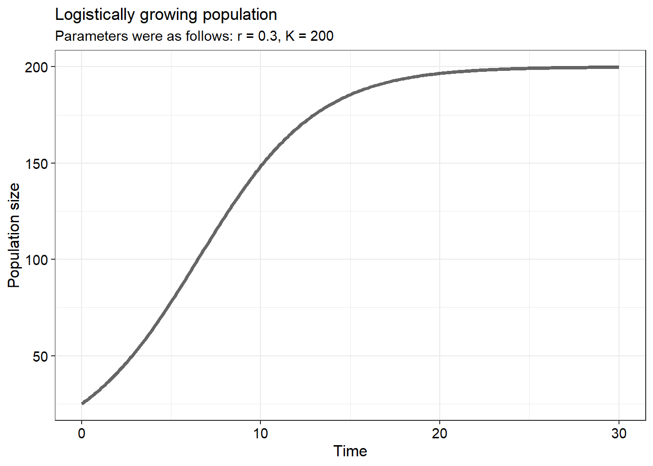
Given the differential equation $\frac{d N}{d t} = r t$ use the desolve package to produce an output resembling the following figure (10)

Following the same instructions as above produce a plot that resembles this output (10)

In your own words describe the three aspects required to calculate the integrals for each time period and how they work together to produce the desired output (9)

Application questions

Some of the more commonly studied and cited examples of predator-prey interactions concern northern hemisphere animals. However, some of the most exciting examples come from Africa. Identify four scientific articles which study predator-prey interactions in Africa. For each article supply

the full citation (1 mark each)
the predator and the prey species (2 marks each)
a five sentence paragraph describing the key findings of the study specifically concerning the interactions between the predators and the prey in relation to the study’s context and aims and objectives (5 marks each)