Plant succession
Introduction
One of the most fundamental ecological phenomenon at a community level is that of succession. Whether it be coral reefs, beaches, grasslands or forests, every habitat type undergoes some kind of succession. Ecological succession is the term used to describe the changes in community composition through time. Generally these time periods range from between a few years to a few millenia during which the community cmposition changes or transitions. These transitions are driven by both biotic and abiotic factors until an equlibrium is reach. Here the community of interest is known as the climax community. This “climax community” is relatively resillient to other factors but the climax community composition can change under intense disturbances. What this intense disturbance might be can vary from habitat to habitat. The type of disturbance can also play important role in directing the successional trends. We will discuss this more later.
Succession can occur under two general sets of conditions - under entirely new habitats and under disturbances. Entirely new habitats are often created after lava depositions resulting from volcanic erruptions or following glacial movements which remove top soil and leave deep, bare scars. These kinds of events result in the almost complete removal of all living individuals and so any new life must arrive from outside of the area. This kind of succession is termed primary succession.
Secondary succession on the other hand occurs under more mild types of disturbances which take place on previously colonised soil. Under heavy burning, cutting or agricultural tilling most or all of the living individuals may be removed from the community but the soil texture, nutrient content and seed bank may remain relatively undisturbed.
Markov Chain succession model
One way ecologists can model succession is through Markov chains or processes. A Markov Chain is often employed in complex statistical proceedures. The basic principle behind Markov Chains is relatively simple, simple enough that it can be implemented during matrix algebra. Markov Chain models are simply models which generate a sequence of events where each instance of the sequence is determined by the state of the preceednig event only. We can apply this idea to successional theory because both primary and secondary succesion describes community transitions through time where the future state of a given system generally generally only depends on the previous state together with the transitional probabilities between two states.
Successional models
Together with the two types of succession there are also three general models of succession; the facilitation model, the tolerance model, and the inhibition model.
To facilitate means to makes something easier which is what the successionally earlier, colonising plants do in this scenario - they alter the environment to make it easier (or facilitate) the colonisation of other organisms which might have been sensitive to the initial conditions. These newer species will likely eventually exclude the initial coloniser species with the community tending towards a climax state.
To tolerate means for one thing to cooccur with something that it does not necessarily like or agree with. This term applies to both the later successional species being tolerated by the initial pioneer species but also that the later successional species are well adapted to any persisting disturbances and so are able to tolerate them.
Finally, to inhibit something means to prevent or reduce something or some event from occurring. In this kind of scenario the pioneer species colonise an environment but rather than shaping it towards some state which would facilitate new climax species from arriving, the environment is shifted towards a state which prevents these species from establishing via some mechanism. Only once this mechanism is broken or removed will later successional species be able (and willing) to colonise the region.
Coral reef succession
For our practical today we will be considering the restoration of a coral reef. Much of the previous reef has been damaged by a variety of important factors. Aspart of an effort to revert this coral reef crisis, coral reef restoration has become an important field in marine ecology. In today’s example we will initially explore the restoration of a damaged coral reef by attempting to simulate passive and active restoration.
After preparing an area simple algae suspended in the ocean might come into contact with this bare substrate, attach to it, and begin to grow. Coral species which release vast amounts of propagules into the ocean may soon also come into contact with the bare substrate, attach to it and begin to grow. Soon what was once a bare substrate is now covered with algae and coral. Perhaps the coral may be such a good competitor that it displaces the algae and becomes entirely dominant. This exclusion of algae by the coral may alter the habitat in such a way that a third species, a seaweed, may be able to establish itself on the bare substrate now that competition for light with the algae has been removed. As these two species, the coral and the seaweed, become more and more dominant the habitat may become so altered that new species such as crustaceans and eventually fish may return to the habitat.
Considering this example we seem to have a successional pathway on our hands:
- A bare substrate
- Establishment of algae
- Establishment of and eventual dominance of coral
- Re-introduction of seaweed and the co-dominance of coral and seaweed
- Re-introduction of crustaceans
- Re-introduction of fish
The probabilities of transitioning from one community state to another can easily be expressed in matrix form. By convention, the top row of the matrix table represents the species occupying the bare substrate surface at some time \(t\). The left most column then represents the successional state to which the community at time \(t\) can transition to at time \(t+1\). The numerical values that make up the matrix would then indicate the probabilities that a given area would shift from being occupied by one species to the next.
| Species at \(t+1\) | Bare substrate | Algae | Coral | Seaweed | Crustaceans | Fish |
|---|---|---|---|---|---|---|
| Bare substrate | 0.1 | 0.1 | 0.05 | 0.025 | 0.025 | 0.025 |
| Algae | 0.7 | 0.6 | 0.15 | 0.075 | 0.025 | 0.025 |
| Coral | 0.1 | 0.1 | 0.5 | 0.3 | 0.3 | 0.3 |
| Seaweed | 0.05 | 0.1 | 0.2 | 0.4 | 0.3 | 0.3 |
| Crustaceans | 0.05 | 0.05 | 0.05 | 0.1 | 0.2 | 0.15 |
| Fish | 0 | 0.05 | 0.05 | 0.1 | 0.15 | 0.2 |
Simply reading off these probabilities is an easy way to understand what is going on here. Consider the algae transitions to time \(t+1\) for example. There is a 10% chance that patches of bare substrate dominated by algae will either revert to bare substrate or transition to coral or seaweed based communities while there is a 60% chance that algae patches will remain algae patches. It is important that the sum of each column adds to 1. This because we are considering relative or proportional abundance rather than total abundance, we are studying the surface of the bare substrate not the overall community productivity, for instance.
To incorporate this transition matrix into our study community we need to know the initial community composition of the bare substrate Suppose our initial community looked like this
insert example figure here
we could describe this in what is known as a state vector - a one dimentional matrix as follows:
\[ S_t = \left[ \begin{array}{c} 0.7 \\ 0.2 \\ 0.05 \\ 0.05 \\ 0 \\ 0 \end{array} \right] \]
Then to calculate the community composition at time \(t+1\) we would then multiply this initial state vector by the transitional matrix \(T\):
\[ T = \left[ \begin{array}{cccccc} 0.1 & 0.1 & 0.05 & 0.025 & 0.025 & 0.025 \\ 0.7 & 0.6 & 0.15 & 0.075 & 0.025 & 0.025 \\ 0.1 & 0.1 & 0.5 & 0.3 & 0.3 & 0.3 \\ 0.05 & 0.1 & 0.2 & 0.4 & 0.3 & 0.3 \\ 0.05 & 0.05 & 0.05 & 0.1 & 0.2 & 0.15 \\ 0 & 0.05 & 0.05 & 0.1 & 0.15 & 0.2 \end{array} \right] \]
Such that:
\[S_{t+1} = T \times s_t\]
To illustrate this with our specific example,
\[ S_{t+1} = \left[ \begin{array}{cccccc} 0.1 & 0.1 & 0.05 & 0.025 & 0.025 & 0.025 \\ 0.7 & 0.6 & 0.15 & 0.075 & 0.025 & 0.025 \\ 0.1 & 0.1 & 0.5 & 0.3 & 0.3 & 0.3 \\ 0.05 & 0.1 & 0.2 & 0.4 & 0.3 & 0.3 \\ 0.05 & 0.05 & 0.05 & 0.1 & 0.2 & 0.15 \\ 0 & 0.05 & 0.05 & 0.1 & 0.15 & 0.2 \end{array} \right] \times \left[ \begin{array}{c} 0.7 \\ 0.2 \\ 0.05 \\ 0.05 \\ 0 \\ 0 \end{array} \right] \]
Let’s see how this particular community will change after 15 years:
library(tidyverse)## -- Attaching packages ------------------------------------------ tidyverse 1.2.1.9000 --## v ggplot2 3.0.0.9000 v purrr 0.2.5
## v tibble 1.4.2 v dplyr 0.7.7
## v tidyr 0.8.1 v stringr 1.3.1
## v readr 1.1.1 v forcats 0.3.0## -- Conflicts -------------------------------------------------- tidyverse_conflicts() --
## x dplyr::filter() masks stats::filter()
## x dplyr::lag() masks stats::lag()library(viridis)## Loading required package: viridisLiteyears <- 15
St <- matrix(data = c(0.7, 0.2, 0.05, 0.05, 0, 0, rep(0, 6*(years-1))), ncol = years)
T <- matrix(data = c(0.1, 0.7, 0.1, 0.05, 0.05, 0,
0.1, 0.6, 0.1, 0.1, 0.05, 0.05,
0.05, 0.15, 0.5, 0.2, 0.05, 0.05,
0.025, 0.075, 0.3, 0.4, 0.1, 0.1,
0.025, 0.025, 0.3, 0.3, 0.2, 0.15,
0.025, 0.025, 0.3, 0.3, 0.15, 0.2),
ncol = 6)
St[1,1]*T[1,]## [1] 0.0700 0.0700 0.0350 0.0175 0.0175 0.0175i <- 2
j <- 1
for (i in 2:15) {
for (j in 1:6) {
St[j,i] <- sum(St[,i-1] * T[j,])
}
}
St[j,i] <- sum(St[,1] * T[1,])
abund_df <- as.data.frame(t(St))
colnames(abund_df) <- c("Rock", "Algae", "Coral", "Seaweed", "Crustaceans", "Fish")
abund_df$Year <- seq(from = 1, to = 15, by = 1)
abund_df <- abund_df %>% gather(key = "Species", value = "Abundance", -Year)
abund_df$Species <- factor(abund_df$Species, levels = c("Rock",
"Algae",
"Coral",
"Seaweed",
"Crustaceans",
"Fish"))
ggplot(abund_df) +
geom_line(aes(x = Year, y = Abundance, colour = Species), size = 1) +
scale_color_viridis(discrete = TRUE) +
theme_bw() +
theme(axis.title = element_text(colour = "black",
size = 12),
axis.text = element_text(colour = "black",
size = 11),
strip.text = element_text(colour = "black",
size = 12)) +
labs(x = "Time", y = "Abundance (%)", colour = "Species")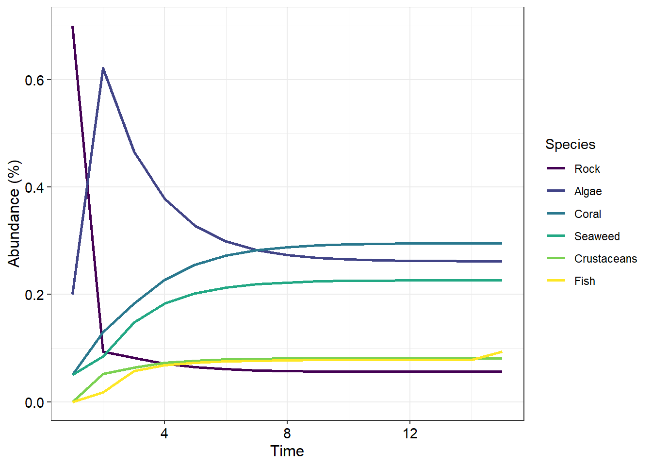
Download the community succession app here and complete the prac worksheet questions.
Worksheet questions
Question 1
In a similar manner to how stage transitions are depicted using diagrams as with stage structured population growth, loop diagrams can be used to described community succession transition probabilities. Without altering any of the parameters of the app draw a diagram describing these transition probabilities between stages (12)
Question 2
Describe the parameter conditions required for
- inhibition of later colonists by early colonists (4)
- tolerance and coexistance by all colonists (4)
- facilitation of crustaceans by the earlier colonists and inhibition of fish (4)
Coding questions
Study this article and develop the code to produce a figure which describes the secondary succession from a generic agricultural cropland to a generic grassland grassland (20)
Application questions
For each of the three types of succession (facilitation, tolerance, inhibition) identify three examples from the scientific literature. Cite the article and give a short description of the types of species/communities involved and a brief discussion on what makes this an example of this particular kind of succession (12)
An important topic in successional theory is that of “alternate stable states”. This area of research attempts to describe how a community will transition based on past disturbances and anthropogenic management influences. Study this article (and any other key articles you can find relating to the topic) to learn about the origins of the idea and then write a short essay (approximately 500 words and at least 5 references) explaining the idea in your own words. On top of that give four examples of this idea being applied to succession in African ecosystems (15)
Describe how you might incorporate alternate stable state theory into your successional model (8)